Reports and Visualisation
Data and analysis results can be viewed in a number of ways in FSL-MRS, and at all stages of processing.
There are five ways of visualising/interacting with MRS data in FSL-MRS:
Quick glance (human-readable, non-interactive)
CSV files (human- and machine-readable)
HTML reports (fairly interactive)
FSLeyes (highly interactive)
SVS results dashboard (interactive)
1. Quick glance
The first thing one might want to do when given a FID file or simulated spectra is to have a quick look at the spectra to see if they look like one would expect. To get a sense of the dimensionality and basic status of the data run mrs_tools info for a quick text summary. FSL-MRS then provides a light-weight script (mrs_tools vis) to quickly visualise the MRS or MRSI data. For example, running mrs_tools vis on the provided example SVS data:
mrs_tools vis example_usage/example_data/metab.nii
gives the following basic plot:

Note that the reason mrs_tools vis “knows” how to scale the x-axis is that the relevant information is stored in the NIfTI-MRS MRS header extension (namely the dwell time and the central frequency).
mrs_tools vis can also visualise a folder of mrs data:
mrs_tools vis ./converted_data_dir/

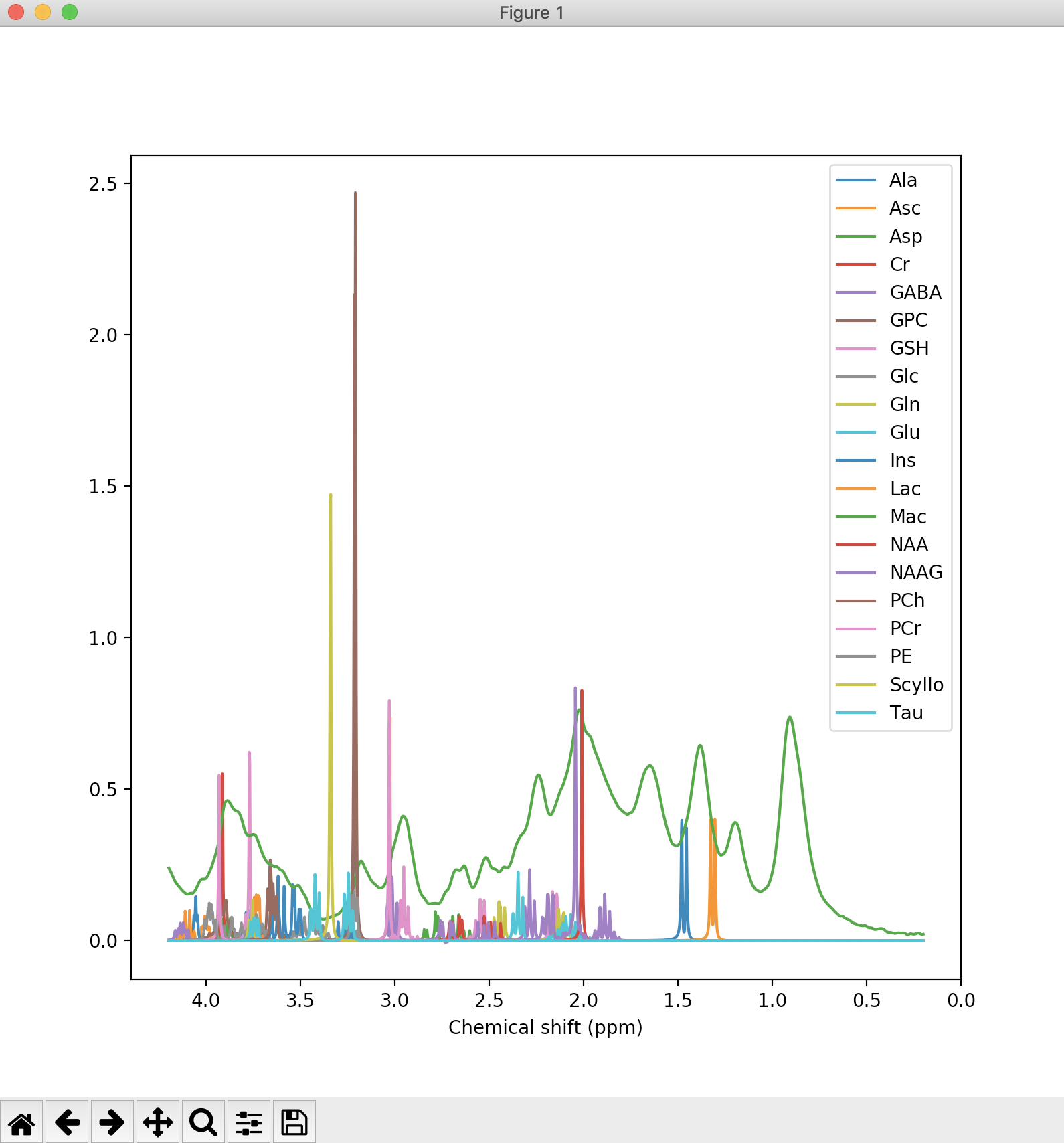
We can also run mrs_tools vis to visualise the metabolite basis. Again below we do so for the simulated basis provided with the example data:
mrs_tools vis example_usage/example_data/steam_11ms/
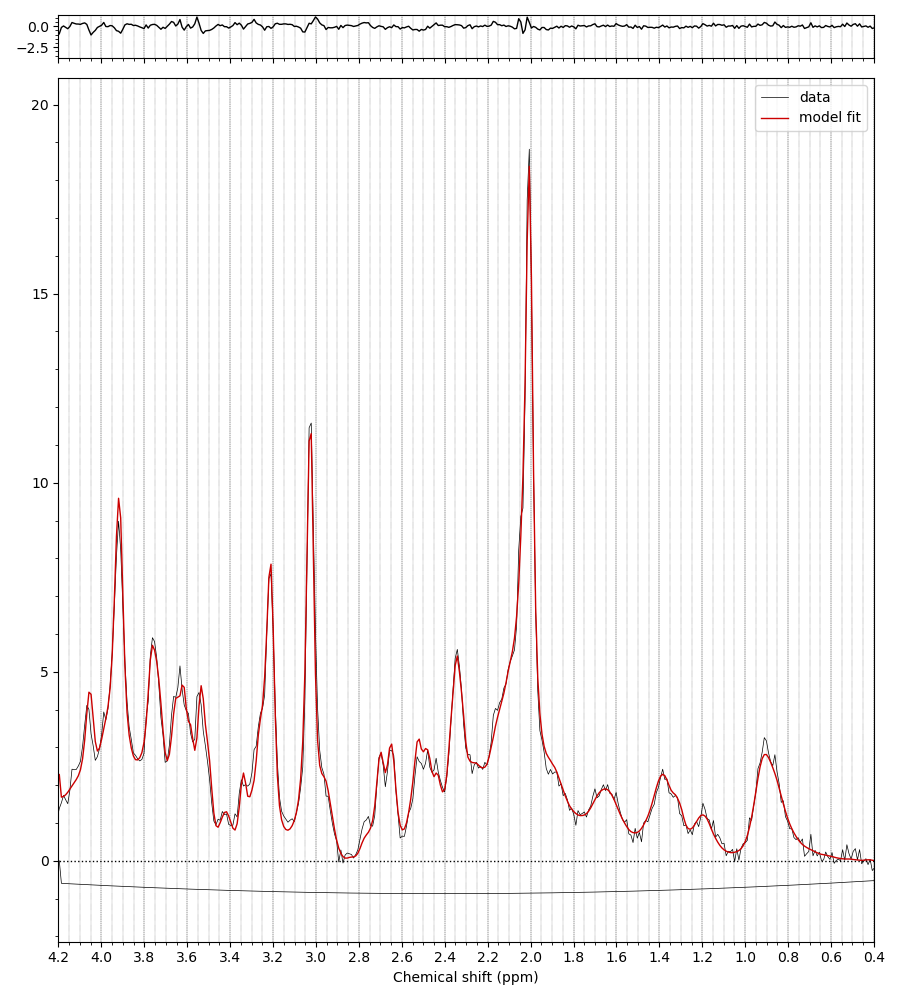
Additionally, the fsl_mrs and fsl_mrsi wrapper scripts output a PNG file (fit_summary.png) that summarises the fitting (overlays the FID spectrum, baseline, and model prediction). An example such file is shown below:
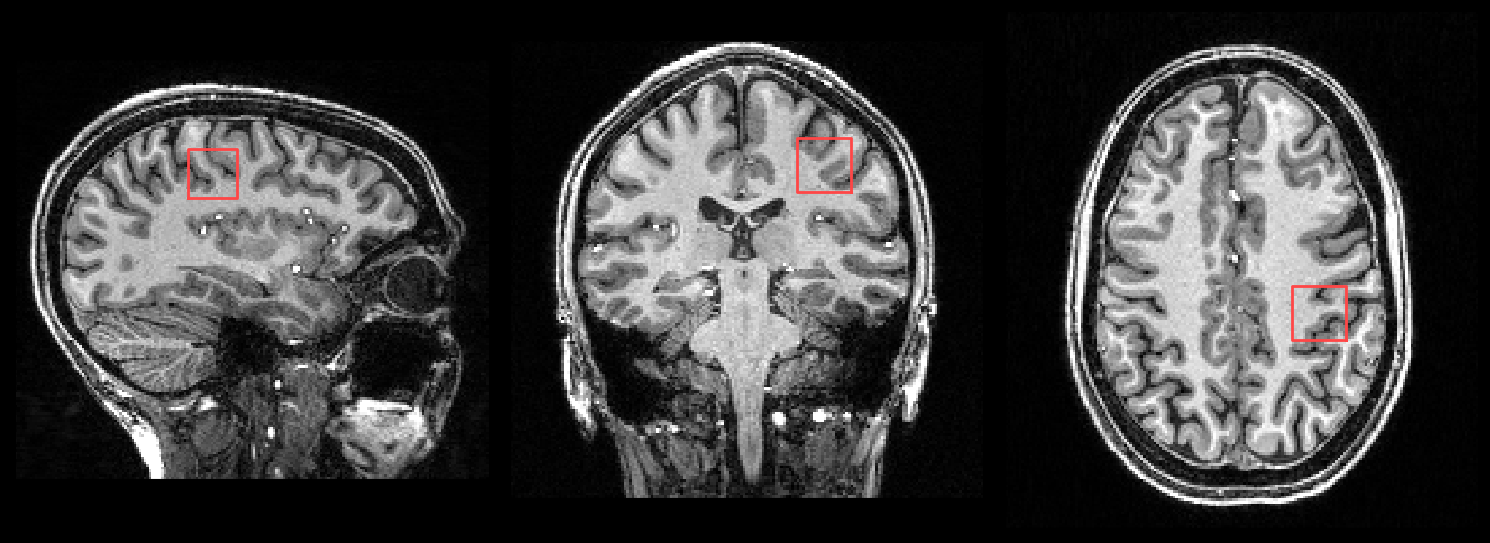
When a T1 image is provided, the SVS voxel location is also shown both the HTML reports and in a PNG file (voxel_location.png):
2. CSV files
The FSL-MRS wrapper scripts generate several CSV files containing the fitted concentrations, QC values, and MCMC samples (when using the flag --algo MH). These can be read out by another tool (e.g. Pandas) for further analyses/statistics.
3. HTML Reports
FSL-MRS can generate interactive HTML reports either through the wrapper scripts (fsl_mrs and fsl_mrsi) or from within a python script or IPython/Jupyter Notebook session. The interactive visualisation uses the Plotly library and allows one to interrogate the FID data and fitting, as well as looking at the correlation between fitted concentrations, uncertainties, and visualising single metabolite spectra alongside the data.
4. FSLeyes
A very powerful way to visualise MRS data is using the MRS plugin for FSLeyes. This is particularly useful for MRSI data, where we can simultaneously view the spectrum and fitted model alongside the anatomical image and interactively navigate from voxel to voxel.
The plugin, which now comes as standard with FSL, has detailed online documentation.
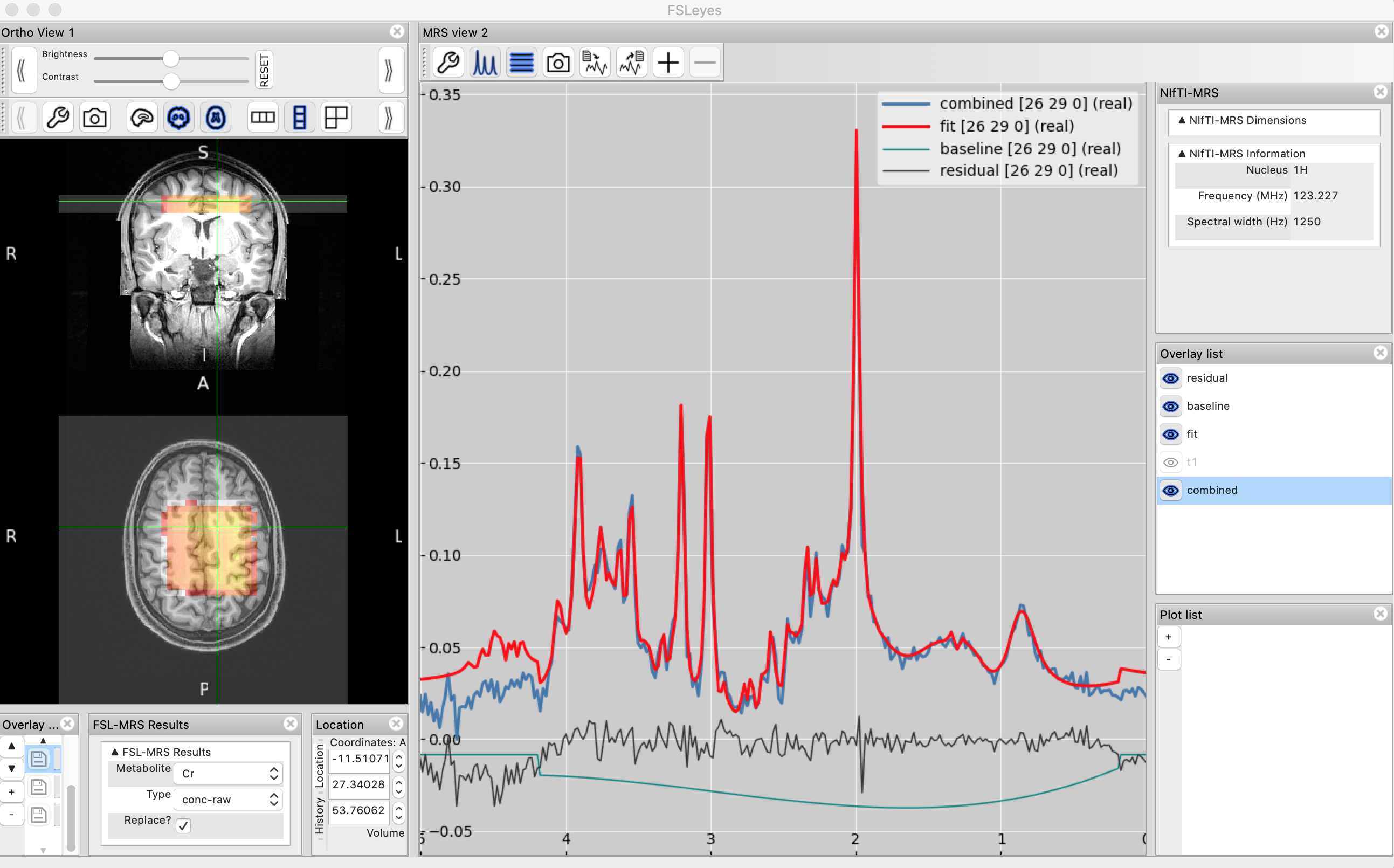
Below are instructions for loading and configuring FSLeyes to work with an MRSI data set. Say the input FID (used for fitting) is FID_Metab.nii.gz and the output from fsl_mrsi is a folder called mrsi_output. You can load these data into FSLeyes with:
fsleyes -smrs FID_Metab.nii.gz T1.nii &
Subsequently navigate to the Tools menu and select the LoadLoad FSL-MRS fit option. Select the mrsi_output folder to load.
You should be able to see something like this:
1. SVS results dashboard
Warning: experimental / new feature
The results from multiple single voxel (SVS) fits can be viewed on a single webpage by using the fsl_mrs_summarise command. For example:
fsl_mrs_summarise dir results_dir/
or
fsl_mrs_summarise list results.txt
Where results_dir/ contains sub-directories of results generated by the fsl_mrs command, or results.txt contains a line-separated list of directories.
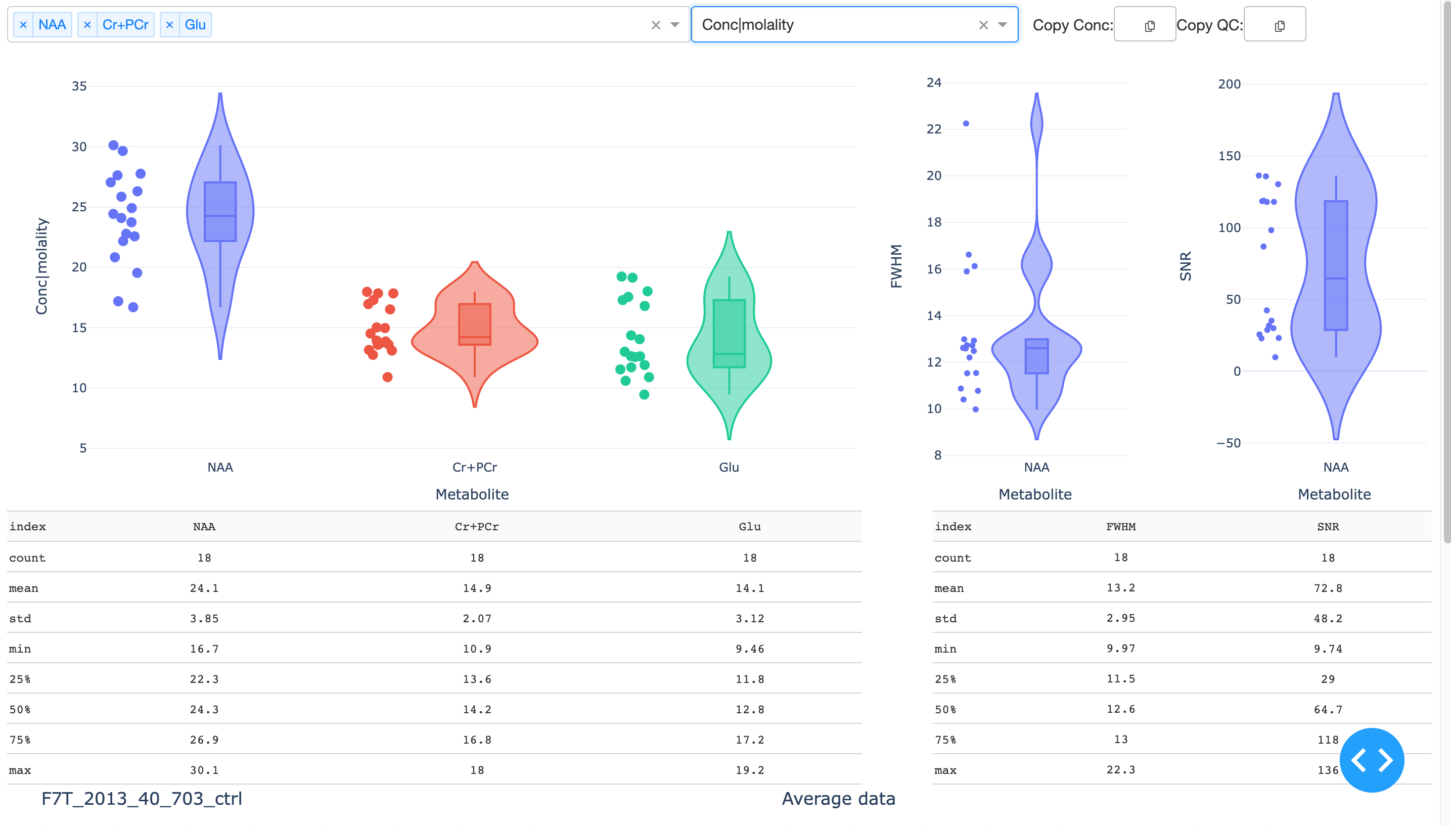
This generates an interactive Dash app that displays metabolite concentrations, uncertainties, and QC parameters (SNR and linewidths). Sumamry statistics are given in table form below.
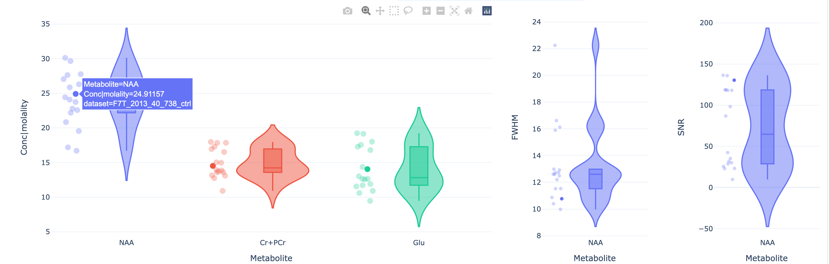
By selecting one of the plotted datasets, the data + fit is displayed lower in the page.
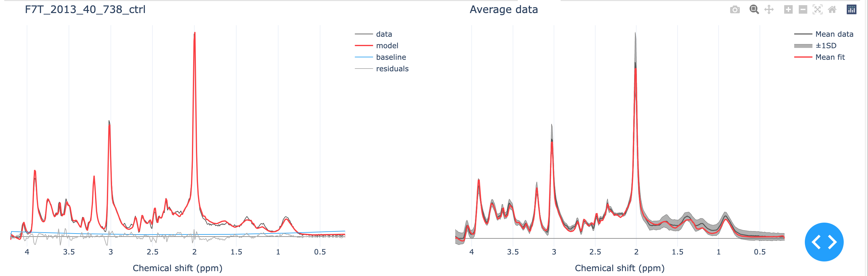
The single dataset + fit is displayed next to the mean (±1SD) data and fit.