Code explanation
Interested in generating hybrid FODs with own diffusion MRI and microscopy data? Here we provide details of the method alongside important snippets of code. The full code is made openly at https://git.fmrib.ox.ac.uk/srq306/hybrid_microscopy_dmri.
Diffusion MRI orientation
Diffusion MRI (dMRI) orientations were estimated using the Ball and stick model in FSL. The signal decay of the diffusion was modelled by an isotropic compartment (Ball) and multiple restricted compartments for fibre orientation (Stick).
dMRI was analysed to estimate ≤ 3 fibre populations with 50 orientation estimates (samples) per population.
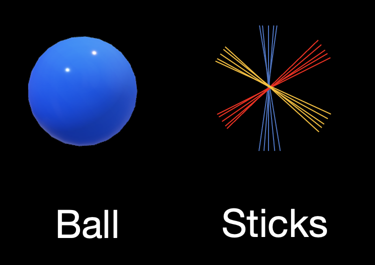
Fibre populations with signal fractions less than 0.05 were removed. Details of ball and stick model output can be found here
Microscopy orientation
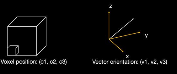
First, the microscopy orientation was registered to the dMRI space with TIRL and FSL FLIRT. The voxel coordinate for each microscopic pixel was then described by x, y, z coordinates in the diffusion mri space (c1,c2,c3). The fiber orientation was represented by a 3D vector (v1,v2,v3).
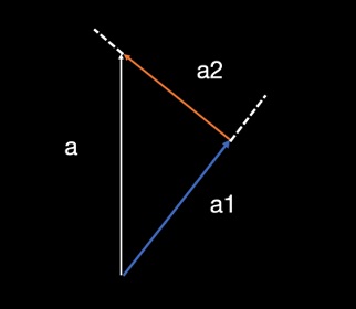
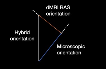
Second, to facilitate a comparison between the 3D dMRI fibre orientation and 2D microscopy orientation, the dMRI orientation (a) was projected onto the 2D microscopy plane (a1) and onto the normal vector of the plane (a2). Next, the angle difference between the projected BAS orientation and the microscopy orietnation was calculated.
function out = project(v,n)
%Ensure norm is unit
n = n./vecnorm(n,2,2);
% Find vector projection
a1 = sum(v.*n,2).*n;
% i.e. the vector projected onto the plane
a2 = v-a1;
out.a1 = a1;
out.a2 = a2;
end
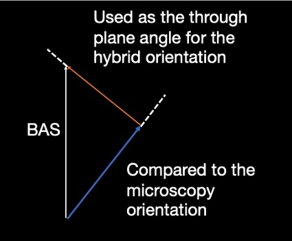
Third, the BAS sample with the smallest angle to the microscopy orientation on the microscopy plane was selected. The through plane angle of the diffusion sample was used for the hybrid orientation reconstruction.
 % Record smallest angle between vector and any dyad sample
[~,indd] = max(cosangsqrd,[],2,'omitnan');
linearind = sub2ind(size(cosangsqrd),1:size(cosangsqrd,1),indd'); %'
angg = acos(sqrt(cosangsqrd(linearind)));


a1 = reshape(a1,[],3);
a2 = reshape(a2,[],3);

% Output dyad sample most closely associated with each micro orientation
selected.a1 = a1(linearind,:);
selected.a2 = a2(linearind,:);
selected.ang = angg;
selected.ind = indd;
Hybrid orientation
We merged the in-plane orientation from the microscopy data with the through-plane orientation of the best matched diffusion sample to create a 3D hybrid orientation.
micro.vect3D = tmp.inplane.*vecnorm(tmp.a2,2,2)+tmp.a1;
micro.vect3D = reshape(micro.vect3D,size(micro.inplane));
We then combine the hybrid fibre orientations over a local neighbourhood with the size of the desired voxel to create a hybrid fibre orientation distribution (FOD). For each voxel, the orientation was compared to a 3D vector set (256 directions evenly distributed across a sphere) to populate a 3D frequency histogram.
% For each voxel in hr space, extract fibre orientations, compare
% to directions in 'vectors' and populate frequency histogram
VV = unique(voxind);
VV(isnan(VV)) = [];
for w = 1:numel(VV)
    v = VV(w);
    if roimask_us(v)==1
        ind = voxind==v;
        if sum(ind)>0
            out = hist_sphere(micro.vect3D(ind,:),vectors);
            count(v,:) = count(v,:)+out.count;
        end
    end
    if mod(w,500)==0, disp([num2str(w) '/' num2str(numel(VV))]); end
 end
Spherical harmonics were then fitted to to the frequency histogram to generate our hybrid FODs.
% Fit SH coeffs to frequency matrix
if mrtrixflag
    vectors(1,:) = -vectors(1,:);
    disp('LR flip for mrtrix')
end

SHmat = SH_transform(vectors,8); % get the spherical harmonics basis
SHmat_pinv = pinv(SHmat);
Ncoeffs = size(SHmat,2);

% Normalise hsitogram by number of pixels in each voxel
countn = count./sum(count,2);
coeffs = SHmat_pinv*countn';
SH_3D = reshape(coeffs',s1,s2,s3,Ncoeffs);
count_3D = reshape(count,s1,s2,s3,256);